Tutorial 3. Use SEDR to do batch integration.
Here we use 3 sections from DLPFC data to show the ability of SEDR to integrate batches for the same tissue with the same techniques.
[1]:
import os
import torch
import numpy as np
import pandas as pd
import scanpy as sc

import matplotlib.pyplot as plt
import seaborn as sns

import warnings
warnings.filterwarnings('ignore')

from pathlib import Path
from tqdm import tqdm
[2]:
import SEDR
[3]:
data_root = Path('../data/DLPFC/')

proj_list = [
    '151673', '151674', '151675'
]
Combining datasets
Input of SEDR includes an AnnData object that contains the spatial transcriptomics data and a graph dictionary that contains the neighborhood graph. When combining two datasets, the AnnData objects are directly concatenated. For neighborhood graphs, we follow the following algorithm.
Let \(A^k\) and \(Z_f^k\) denote the adjacency matrix and deep gene representation of spatial omics k, we then create a block-diagonal adjacency matrix \(A^k\) and concatenate the deep gene representation in the spot dimension, as:

where K is the number of spatial omics.
[4]:
for proj_name in tqdm(proj_list):
    adata_tmp = sc.read_visium(data_root / proj_name)
    adata_tmp.var_names_make_unique()

    adata_tmp.obs['batch_name'] = proj_name


    ##### Load layer_guess label, if have
    df_label = pd.read_csv(data_root / proj_name / 'metadata.tsv', sep='\t')
    adata_tmp.obs['layer_guess'] = df_label['layer_guess']
    adata_tmp= adata_tmp[~pd.isnull(adata_tmp.obs['layer_guess'])]

    graph_dict_tmp = SEDR.graph_construction(adata_tmp, 12)

    if proj_name == proj_list[0]:
        adata = adata_tmp
        graph_dict = graph_dict_tmp
        name = proj_name
        adata.obs['proj_name'] = proj_name
    else:
        var_names = adata.var_names.intersection(adata_tmp.var_names)
        adata = adata[:, var_names]
        adata_tmp = adata_tmp[:, var_names]
        adata_tmp.obs['proj_name'] = proj_name

        adata = adata.concatenate(adata_tmp)
        graph_dict = SEDR.combine_graph_dict(graph_dict, graph_dict_tmp)
        name = name + '_' + proj_name
100%|██████████| 3/3 [00:06<00:00, 2.10s/it]
Preprocessing
[5]:
adata.layers['count'] = adata.X.toarray()
sc.pp.filter_genes(adata, min_cells=50)
sc.pp.filter_genes(adata, min_counts=10)
sc.pp.normalize_total(adata, target_sum=1e6)
sc.pp.highly_variable_genes(adata, flavor="seurat_v3", layer='count', n_top_genes=2000)
adata = adata[:, adata.var['highly_variable'] == True]
sc.pp.scale(adata)

from sklearn.decomposition import PCA  # sklearn PCA is used because PCA in scanpy is not stable.
adata_X = PCA(n_components=200, random_state=42).fit_transform(adata.X)
adata.obsm['X_pca'] = adata_X
Training SEDR
[6]:
sedr_net = SEDR.Sedr(adata.obsm['X_pca'], graph_dict, mode='clustering', device='cuda:3')
using_dec = False
if using_dec:
    sedr_net.train_with_dec()
else:
    sedr_net.train_without_dec()
sedr_feat, _, _, _ = sedr_net.process()
adata.obsm['SEDR'] = sedr_feat
100%|██████████| 200/200 [00:09<00:00, 21.43it/s]
use harmony to calculate revised PCs
[7]:
import harmonypy as hm

meta_data = adata.obs[['batch']]

data_mat = adata.obsm['SEDR']
vars_use = ['batch']
ho = hm.run_harmony(data_mat, meta_data, vars_use)

res = pd.DataFrame(ho.Z_corr).T
res_df = pd.DataFrame(data=res.values, columns=['X{}'.format(i+1) for i in range(res.shape[1])], index=adata.obs.index)
adata.obsm[f'SEDR.Harmony'] = res_df
2024-11-06 14:34:39,484 - harmonypy - INFO - Computing initial centroids with sklearn.KMeans...
2024-11-06 14:34:41,350 - harmonypy - INFO - sklearn.KMeans initialization complete.
2024-11-06 14:34:41,386 - harmonypy - INFO - Iteration 1 of 10
2024-11-06 14:34:43,146 - harmonypy - INFO - Iteration 2 of 10
2024-11-06 14:34:44,927 - harmonypy - INFO - Iteration 3 of 10
2024-11-06 14:34:46,724 - harmonypy - INFO - Iteration 4 of 10
2024-11-06 14:34:48,567 - harmonypy - INFO - Iteration 5 of 10
2024-11-06 14:34:50,444 - harmonypy - INFO - Iteration 6 of 10
2024-11-06 14:34:51,926 - harmonypy - INFO - Converged after 6 iterations
Visualizing
UMAP
[8]:
sc.pp.neighbors(adata, use_rep='SEDR.Harmony', metric='cosine')
sc.tl.umap(adata)
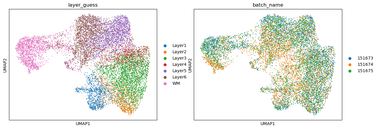
[9]:
sc.pl.umap(adata, color=['layer_guess', 'batch_name'], show=False)
[9]:
[<Axes: title={'center': 'layer_guess'}, xlabel='UMAP1', ylabel='UMAP2'>,
 <Axes: title={'center': 'batch_name'}, xlabel='UMAP1', ylabel='UMAP2'>]
LISI score
[10]:
ILISI = hm.compute_lisi(adata.obsm['SEDR.Harmony'], adata.obs[['batch']], label_colnames=['batch'])[:, 0]
CLISI = hm.compute_lisi(adata.obsm['SEDR.Harmony'], adata.obs[['layer_guess']], label_colnames=['layer_guess'])[:, 0]
[11]:
df_ILISI = pd.DataFrame({
    'method': 'SEDR',
    'value': ILISI,
    'type': ['ILISI']*len(ILISI)
})


df_CLISI = pd.DataFrame({
    'method': 'SEDR',
    'value': CLISI,
    'type': ['CLISI']*len(CLISI)
})

fig, axes = plt.subplots(1,2,figsize=(4, 5))
sns.boxplot(data=df_ILISI, x='method', y='value', ax=axes[0])
sns.boxplot(data=df_CLISI, x='method', y='value', ax=axes[1])
axes[0].set_ylim(1, 3)
axes[1].set_ylim(1, 7)
axes[0].set_title('iLISI')
axes[1].set_title('cLISI')

plt.tight_layout()

[ ]:
[ ]:
[ ]:
[ ]: